07 · Networks and multi-model simulations: water that leaves the grid and comes back#
In tutorials 01 to 06 every external term was an end point: water entering through recharge or a stream started there, and water leaving through a drain or a well was gone. Real models are less tidy. A drain may hand its water to a stream through the water mover (MVR), the stream may lose that water back to the aquifer a kilometre away, and a pumping well there may take it. A multi-aquifer well (MAW) takes water from one layer and loses part of it into another through its borehole. And a large model may be split into several models joined by exchanges.
In each case water passes through something that is not a model cell. If the trace stops at the cell boundary, the route is cut: water handed to the stream looks lost, and water leaking from the stream looks like a new source with no history. gwsource can instead read these features as nodes of the same graph, so the full-mixing trace follows the water through them.
This tutorial covers three such cases:
Stream and mover (SFR + MVR): drains feed the stream of tutorial 01, which leaks to the aquifer near the well. First a trace on the cells alone, then with one node per stream reach and the mover transfers as edges, following drain → MVR → stream → aquifer → well.
A multi-aquifer well (MAW) screened in three layers, which moves water from layer 1 to layer 3 through its borehole.
A split model: the quickstart model cut into three models joined by GWF-GWF exchanges gives the same answer as the single model.
It closes with the MODFLOW 6 options these features need and the current limitations.
Runtime: about 3 seconds (the last code cell prints the measured time). Prerequisites: tutorial 01 (fraction through, volume from); the tutorial README for setup.
Settings#
All settings live in this first cell. Later cells use only these names and what earlier cells return. Workspaces go to tutorials/_work/07_networks_multimodel/ (git-ignored, recreated on every run). The shared builders are in herebedragons.py. A route diagram, a cross-section and two small tables specific to this tutorial are in helpers.py, next to this notebook.
import sys
import time
from pathlib import Path

import flopy
import matplotlib.pyplot as plt
import numpy as np
import pandas as pd

sys.path.insert(0, str(Path.cwd().parent))  # tutorials/ holds the shared helpers
sys.path.insert(0, str(Path.cwd()))  # this folder holds helpers.py
import herebedragons as hbd  # noqa: E402
import helpers  # noqa: E402  (this tutorial's route diagram, cross-section and tables)

import gwsource as gs  # noqa: E402

T_START = time.perf_counter()  # for the runtime printed at the end
WORK = hbd.work_dir("07_networks_multimodel", clean=True)  # tutorials/_work/... (git-ignored)
MF6 = hbd.mf6_exe()  # <repo>/bin/mf6
WELL = "supply_well"  # boundname of the supply well traced in every part
SPLIT_ROW, SPLIT_COL = 20, 20  # the split: west half, north-east and south-east quarters

plt.rcParams.update({"figure.dpi": 80, "figure.figsize": (7.0, 5.5)})
print(f"gwsource {gs.__version__}, FloPy {flopy.__version__}")
gwsource 0.0.1, FloPy 3.12.0.dev0
1. A stream fed by drains#
hbd.build_stream_mover is the quickstart model of tutorial 01 (2 km × 2 km, 50 m cells, recharge, constant-head west edge, supply well in row 21, column 29) with two drains added. The model’s stream (SFR) has one reach per row down column 31 and flows north to south. No water enters it from upstream. Its water is groundwater that seeps in through the stream bed. The variant adds:
two drains west of the stream (rows 9 and 23, column 15);
the water mover (MVR), which hands the drains’ outflow to the first (northern) reach: 80 % of
drain_a’s water and all ofdrain_b’s. The rest ofdrain_a’s water leaves the model.
So drained groundwater is carried to the head of the stream and flows south with it. The reaches next to the well lose part of the stream’s water to the aquifer, and the supply well may pump it. The model saves the SFR and MVR budgets to their own files (BUDGET FILEOUT), which section 3 needs. Rows and columns are counted from 1, from the north-west corner, as in tutorials 01 to 03.
stream = hbd.build_stream_mover(WORK / "stream", MF6)
cells_only = gs.read_step(stream.ws, boundnames=True)

LABELS = {
    "WEL": "supply well", "DRN": "drains (leaving the model)", "DRN:DRN-TO-MVR": "drains (to the mover)",
    "RCH": "recharge", "CHD": "west edge", "SFR": "stream leakage / seepage",
}
rows = {}
for index, name in enumerate(cells_only.package_names):
    q = cells_only.term_flow[cells_only.term_package == index]
    rows[LABELS.get(name, name)] = {"in (m3/d)": q[q > 0].sum(), "out (m3/d)": 0.0 - q[q < 0].sum()}
display(pd.DataFrame(rows).T.round(1))
print(f"the two drain records together: {rows[LABELS['DRN']]['out (m3/d)'] + rows[LABELS['DRN:DRN-TO-MVR']]['out (m3/d)']:.1f} m3/d")
| in (m3/d) | out (m3/d) | |
|---|---|---|
| supply well | 0.0 | 800.0 |
| drains (leaving the model) | 0.0 | 21.6 |
| drains (to the mover) | 0.0 | 201.0 |
| recharge | 1950.0 | 0.0 |
| west edge | 456.7 | 0.0 |
| stream leakage / seepage | 125.8 | 1509.9 |
the two drain records together: 222.6 m3/d
This is the budget of the aquifer cells. Recharge (1950 m³/d) and the west edge (about 460 m³/d) bring water in. The stream leaks about 126 m³/d into the aquifer and takes about 1510 m³/d back. The drains take about 223 m³/d, of which 201 m³/d is handed to the mover: MF6 writes two records per drain, DRN for the part that leaves the model and DRN-TO-MVR for the moved part.
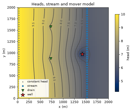
The heads show the effect of the drains and the well. Each drain pulls the contours west around it. The supply well draws the water table down next to the stream, below the stream’s stage.
heads = flopy.utils.HeadFile(str(stream.head_file)).get_data().ravel()
ax = hbd.plot_cells(stream.grb_file, cells_only, heads, cmap="cividis", title="Heads, stream and mover model",
                    label="head (m)")
hbd.add_contours(ax, stream.grb_file, cells_only, heads, np.arange(4.0, 10.5, 0.5), colors="0.3", fmt="%.1f")
plt.show()
2. Trace on the cells alone: the stream is an opaque source#
gs.read_step reads the aquifer cells only (as in tutorials 01 to 06). Every SFR record in the aquifer budget becomes an external term of its cell: positive (stream → aquifer) is a source, negative (aquifer → stream) a sink. The DRN-TO-MVR records are sinks too. The route drain → mover → stream → aquifer is cut in two places.
back_off = gs.backward(cells_only, {WELL: gs.select(cells_only, boundnames=[WELL])})
F_off = back_off.fraction_through[WELL]
display(hbd.volume_from_table(back_off, WELL).round({"volume_from": 1, "share": 3}))
drain_nodes = stream.info["drain_nodes"]  # {boundname: cell}
print("fraction through in the drain cells:", {b: round(float(F_off[n]), 3) for b, n in drain_nodes.items()})
| volume_from | share | |
|---|---|---|
| source | ||
| RCH | 536.6 | 0.671 |
| CHD | 137.6 | 0.172 |
| SFR | 125.8 | 0.157 |
fraction through in the drain cells: {'drain_a': 0.0, 'drain_b': 0.0}
On the cells alone, about a sixth of the well’s water (about 126 m³/d) is “SFR”: it leaked from the stream, and the trace cannot say where the stream got it. The drain cells have \(F = 0\): their water leaves through the drain and, as far as this graph knows, is gone. Both statements describe the graph. Neither describes where the water goes.
3. Open the simulation with package nodes#
gs.open_simulation(ws, package_nodes=("SFR",)) reads the same model as one global graph: first the model cells, then one node per stream reach. The graph is built from three budget files:
aquifer budget: the cell-to-cell flows and the external terms, as before. The aquifer-side SFR records are dropped and replaced by
SFR budget (
BUDGET FILEOUTin SFR): one edge per reach–cell exchange (theGWFrecord) and per reach–reach connection (FLOW-JA-FACE); the reach’s other records (EXT-INFLOW,EXT-OUTFLOW, rainfall, evaporation, runoff) become its source and sink terms, namedSFR:<record>;MVR budget (
BUDGET FILEOUTin MVR): each transfer from a provider (here a drain) to a receiver with nodes (here reach 1) becomes an edge from the drain cell to the reach, and the provider’sDRN-TO-MVRsink is reduced by the same amount.
Package nodes are chosen when the step is read, not in TraceConfig: the graph changes, and every trace, metric and diagnostic then works on the larger graph unchanged.
reader = gs.open_simulation(stream.ws, package_nodes=("SFR",), boundnames=True)
network = reader.read((0, 0))
for block in network.blocks:
    print(f"{block.label:8s} {block.kind:8s} nodes {block.offset}..{block.offset + block.n - 1}")
print("terms:", ", ".join(network.package_names))
print(f"mover transfers routed as edges: {network.notes['mover_routed']:.1f} m3/d")

reaches = network.block("SFR").nodes
exchange = helpers.reach_exchange(network, "SFR")
print(f"stream -> aquifer {exchange['to_cells'].sum():.1f} m3/d, aquifer -> stream (incl. mover) "
      f"{exchange['from_cells'].sum():.1f} m3/d")
display(exchange.loc[[1, 2, 3, 18, 19, 20, 21, 22, 23]].round(1))  # the first reaches and those near the well
stream   model    nodes 0..1599
stream/SFR package  nodes 1600..1639
terms: WEL, DRN, DRN:DRN-TO-MVR, RCH, CHD, SFR:RAINFALL, SFR:EVAPORATION, SFR:RUNOFF, SFR:EXT-INFLOW, SFR:EXT-OUTFLOW, SFR:STORAGE, SFR:FROM-MVR, SFR:TO-MVR
mover transfers routed as edges: 201.0 m3/d
stream -> aquifer 125.8 m3/d, aquifer -> stream (incl. mover) 1710.9 m3/d
| from_cells | to_cells | |
|---|---|---|
| id | ||
| 1 | 249.0 | 0.0 |
| 2 | 48.3 | 0.0 |
| 3 | 48.5 | 0.0 |
| 18 | 11.7 | 0.0 |
| 19 | 0.0 | 6.4 |
| 20 | 0.0 | 31.2 |
| 21 | 0.0 | 52.6 |
| 22 | 0.0 | 30.4 |
| 23 | 0.0 | 5.2 |
The 1600 cells keep their node numbers. The 40 reaches are nodes 1600 to 1639. The table lists, for the first reaches and for the reaches next to the well, the water each receives from cells (seepage, and for reach 1 also the mover edges from the two drain cells) and loses to cells. Reach 1 takes in the 201 m³/d from the drains and about 48 m³/d of seepage. Every reach down to reach 18 gains water from the aquifer. Reaches 19 to 23, next to the well, lose about 126 m³/d to it.
Trace again#
Selection works as before: the well by boundname, a reach term with package="SFR", term="EXT-OUTFLOW".
back_on = gs.backward(network, {WELL: gs.select(network, boundnames=[WELL])})
F_on = back_on.fraction_through[WELL]
n_cells = network.block(stream.name).n  # the model's cells come first in the global numbering

drains = pd.DataFrame(
    {"F, cells only": [F_off[n] for n in drain_nodes.values()],
     "F, with SFR nodes": [F_on[n] for n in drain_nodes.values()]},
    index=pd.Index(list(drain_nodes), name="drain cell"),
)
display(drains.round(3))
print(f"F of reach 1: {F_on[reaches[0]]:.3f}; solver: {back_on.solver_used[0]}, {len(back_on.cycles)} flow loop(s)")
| F, cells only | F, with SFR nodes | |
|---|---|---|
| drain cell | ||
| drain_a | 0.0 | 0.105 |
| drain_b | 0.0 | 0.132 |
F of reach 1: 0.132; solver: topological, 0 flow loop(s)
The drain cells now have \(F \approx 0.105\) and \(0.132\). Their water goes to the mover, the mover sends it to reach 1, and 13.2 % of what passes through reach 1 ends up in the well. drain_b moves all its water, so its \(F\) equals that of reach 1. drain_a moves 80 %, so its \(F\) is \(0.8 \times 0.132 = 0.105\).
The graph has no flow loop: the water that the stream loses near the well is all pumped, so none of it returns to the stream or to a drain. gwsource would solve a graph with flow loops exactly as well (tutorial 04).
The maps below compare the two traces. The right panel shows the \(F\) of each reach, from reach 1 in the north to reach 40 in the south.
points = gs.export.package_points(network)  # {reach node: (x, y) of the cell it exchanges with}
xy = np.array([points[int(n)] for n in reaches])
losing = exchange["to_cells"].to_numpy() > exchange["from_cells"].to_numpy()
fig, axes = plt.subplots(1, 3, figsize=(15.0, 5.0), gridspec_kw={"width_ratios": [1.0, 1.0, 0.38]})
for ax, F, title in ((axes[0], F_off[:n_cells], "Cells only"), (axes[1], F_on[:n_cells], "With SFR nodes and MVR edges")):
    hbd.plot_cells(stream.grb_file, cells_only, F, ax=ax, cmap="viridis", vmin=0.0, vmax=1.0, title=title,
                   label="F (-)", overlay=False)
    hbd.add_contours(ax, stream.grb_file, cells_only, F, (0.1, 0.5), colors="w", linestyles=["--", "-"])
    hbd.overlay_features(ax, stream.grb_file, cells_only, packages=("SFR", "DRN", "WEL"), legend=ax is axes[0])
axes[2].plot(F_on[reaches], xy[:, 1], color="0.5", lw=1.0)
axes[2].scatter(F_on[reaches][losing], xy[losing, 1], color="tab:blue", s=18, label="losing reach")
axes[2].scatter(F_on[reaches][~losing], xy[~losing, 1], color="tab:orange", s=18, label="gaining reach")
axes[2].set_ylim(0.0, stream.spec.ly)
axes[2].set_xlim(0.0, 1.0)
axes[2].set_xlabel("F of the reach (-)")
axes[2].set_ylabel("y of the reach (m)")
axes[2].set_title("Stream reaches")
axes[2].legend(fontsize=8, loc="lower right")
fig.suptitle("Fraction through to the supply well")
fig.tight_layout()
plt.show()

F_reach = pd.Series(F_on[reaches], index=pd.RangeIndex(1, len(reaches) + 1, name="reach"))
last_feeding = int(F_reach[F_reach > 0.0].index.max())  # the last reach that passes water to the well
print(f"F > 0 in every reach from 1 to {last_feeding}: {bool((F_reach.loc[:last_feeding] > 0.0).all())}; "
      f"F of reach 1 {F_reach.loc[1]:.2f}, of reach {last_feeding} {F_reach.loc[last_feeding]:.3f}")
print(f"largest F of reaches {last_feeding + 1} to {F_reach.index[-1]}: {F_reach.loc[last_feeding + 1:].max():.1f}")
print("gaining reaches:", list(F_reach.index[~losing]))
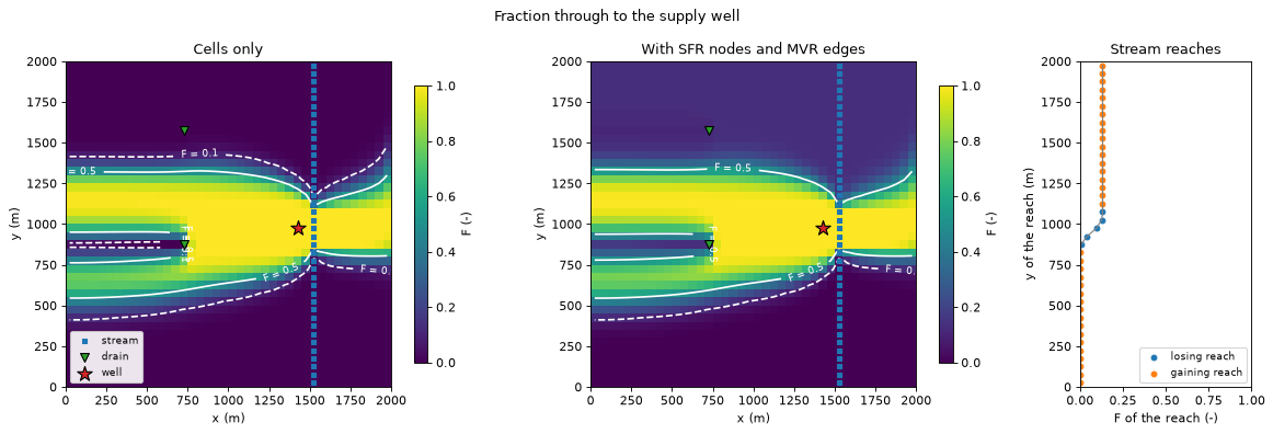
F > 0 in every reach from 1 to 23: True; F of reach 1 0.13, of reach 23 0.006
largest F of reaches 24 to 40: 0.0
gaining reaches: [1, 2, 3, 4, 5, 6, 7, 8, 9, 10, 11, 12, 13, 14, 15, 16, 17, 18, 24, 25, 26, 27, 28, 29, 30, 31, 32, 33, 34, 35, 36, 37, 38, 39, 40]
Left, the capture zone stops at the stream, whose leaking reaches near the well act as sources. Middle, the cells north of the zone and east of the stream now have \(F \approx 0.13\), and so do the drain cells. Their water seeps into reaches 1 to 18 or reaches them through the mover, and 13 % of the stream’s water there leaks to the well further south. Right, \(F\) is the same in reaches 1 to 18, which only gain water. It falls in the losing reaches 19 to 23, from 0.13 to 0.006, and is 0 from reach 24 to reach 40. These lower reaches carry water past the well to the outlet. Close to the well the two maps agree, because the flows are the same; only the bookkeeping at the stream and the drains has changed.
The route, by numbers#
How much of the well’s water came through the drains? Each mover edge carries \(q\) from a drain cell to reach 1. The part that ends in the well is \(q \times F_\text{reach 1}\). The rest of the water the well receives from the stream seeped into the stream from the aquifer.
mover = helpers.edges_between(network, list(drain_nodes.values()), reaches)
mover["drain"] = [b for n in mover["src"] for b, node in drain_nodes.items() if node == n]
mover["F of receiving reach"] = F_on[mover["dst"]]
mover["to well (m3/d)"] = mover["q"] * mover["F of receiving reach"]
display(mover.set_index("drain")[["q", "F of receiving reach", "to well (m3/d)"]].round(3))

via_mover = float(mover["to well (m3/d)"].sum())
q_moved = float(mover["q"].sum())
from_stream = float(back_off.volume_from_by_term[WELL]["SFR"].sum())  # the cells-only "SFR" source
print(f"well water that leaked from the stream:          {from_stream:6.1f} m3/d")
print(f"  of which came through the mover:               {via_mover:6.1f} m3/d")
print(f"  of which seeped into the stream from the cells: {from_stream - via_mover:6.1f} m3/d")
| q | F of receiving reach | to well (m3/d) | |
|---|---|---|---|
| drain | |||
| drain_a | 86.402 | 0.132 | 11.392 |
| drain_b | 114.636 | 0.132 | 15.115 |
well water that leaked from the stream:           125.8 m3/d
  of which came through the mover:                 26.5 m3/d
  of which seeped into the stream from the cells:   99.3 m3/d
The diagram summarises the route. Boxes are nodes or groups of nodes, and \(F\) is the fraction of each node’s water that reaches the well. Arrows carry flows of the model (m³/d). The stream loses 126 m³/d to the aquifer cells below reaches 19 to 23, and the well pumps all of it.
F_drains = F_on[list(drain_nodes.values())]
losing_reaches = F_reach.index[losing]  # reach numbers, counted from 1
seepage = float(exchange["from_cells"].sum()) - q_moved  # aquifer -> stream, without the mover
outlet = -float(network.term_flow[gs.select(network, package="SFR", term="EXT-OUTFLOW").terms].sum())
boxes = {
    "rch": (0.08, 0.72, "recharge on\nthe drained\narea", "#d9f0d3"),
    "drn": (0.25, 0.72, f"2 drain cells\nF = {F_drains.min():.2f}\nand {F_drains.max():.2f}", "#c7e9c0"),
    "mvr": (0.42, 0.72, "water mover\n(MVR)", "#eeeeee"),
    "sfr": (0.59, 0.72, f"stream\nF = {F_on[reaches[0]]:.2f}\nat reach 1", "#9ecae1"),
    "aq": (0.76, 0.72, f"aquifer cells\nbelow reaches\n{losing_reaches.min()} to {losing_reaches.max()}", "#fdd0a2"),
    "well": (0.93, 0.72, f"supply well\n{back_on.destination_inflow[WELL]:.0f} m3/d", "#fc9272"),
    "seep": (0.42, 0.2, "seepage from\nthe aquifer", "#deebf7"),
    "down": (0.76, 0.2, "stream outlet", "#deebf7"),
}
arrows = [
    ("rch", "drn", "drained"),
    ("drn", "mvr", f"{q_moved:.0f}"),
    ("mvr", "sfr", f"{q_moved:.0f}"),
    ("seep", "sfr", f"{seepage:.0f}"),
    ("sfr", "aq", f"{exchange['to_cells'].sum():.0f}"),
    ("sfr", "down", f"{outlet:.0f}"),
    ("aq", "well", f"{from_stream:.0f}"),
]
fig, ax = plt.subplots(figsize=(12.0, 3.6))
helpers.route_diagram(ax, boxes, arrows, half=(0.052, 0.15),
                      title="Drain -> mover -> stream -> aquifer -> well (flows in m3/d)")
plt.show()
print(f"of the {from_stream:.0f} m3/d the well receives from the stream, {via_mover:.0f} m3/d came through the mover")
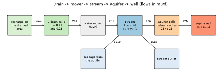
of the 126 m3/d the well receives from the stream, 27 m3/d came through the mover
The well’s water by original source#
With the stream as nodes, the stream is no longer a source: its water is traced back to where it entered the model. The stream has no inflow from upstream, so only recharge and the west edge remain. The second table shows the origin of the water in the losing reaches.
table = pd.concat(
    {"cells only": hbd.volume_from_table(back_off, WELL)["volume_from"],
     "with SFR nodes": hbd.volume_from_table(back_on, WELL)["volume_from"]}, axis=1
).fillna(0.0)
table.loc["  well water that passed through the mover"] = [0.0, via_mover]
table.loc["total"] = [back_off.destination_inflow[WELL], back_on.destination_inflow[WELL]]
display(table.round(1))

forward_on = gs.forward(network, {"recharge": gs.select(network, package="RCH"),
                                  "west edge": gs.select(network, package="CHD")})
origin = pd.DataFrame({g: forward_on.source_fraction[g][reaches[losing]] for g in forward_on.groups},
                      index=pd.Index(losing_reaches, name="water in losing reach, by origin"))
display(origin.round(3))
gain = table["with SFR nodes"] - table["cells only"]
print(f"the {table.loc['SFR', 'cells only']:.1f} m3/d of SFR water: {gain['RCH']:.1f} m3/d recharge and "
      f"{gain['CHD']:.1f} m3/d west-edge water; well water through the mover: {via_mover:.1f} m3/d, "
      f"{via_mover / back_on.destination_inflow[WELL]:.1%} of the pumping")
for name, result, step in (("cells only", back_off, cells_only), ("with SFR nodes", back_on, network)):
    check = gs.diagnostics.backward_closure(step, result, WELL)
    print(f"closure, {name}: volume from {check.lhs:.7f} m3/d, residual term {check.residual_term:.1e} m3/d, "
          f"pumping {check.rhs:.1f} m3/d; relative error {check.relative_error:.1e}, "
          f"{abs(check.error_without_residual) / check.rhs:.1e} without the residual term")
    assert check.relative_error < 1e-8, check
| cells only | with SFR nodes | |
|---|---|---|
| source | ||
| RCH | 536.6 | 636.3 |
| CHD | 137.6 | 163.7 |
| SFR | 125.8 | 0.0 |
| well water that passed through the mover | 0.0 | 26.5 |
| total | 800.0 | 800.0 |
| recharge | west edge | |
|---|---|---|
| water in losing reach, by origin | ||
| 19 | 0.792 | 0.208 |
| 20 | 0.792 | 0.208 |
| 21 | 0.792 | 0.208 |
| 22 | 0.792 | 0.208 |
| 23 | 0.792 | 0.208 |
the 125.8 m3/d of SFR water: 99.7 m3/d recharge and 26.2 m3/d west-edge water; well water through the mover: 26.5 m3/d, 3.3% of the pumping
closure, cells only: volume from 799.9999997 m3/d, residual term -3.2e-07 m3/d, pumping 800.0 m3/d; relative error 1.4e-16, 4.0e-10 without the residual term
closure, with SFR nodes: volume from 799.9999996 m3/d, residual term -4.0e-07 m3/d, pumping 800.0 m3/d; relative error 0.0e+00, 5.0e-10 without the residual term
The 126 m³/d of “SFR” water splits into about 100 m³/d of recharge and about 26 m³/d of west-edge water. That is the mix of the water in the losing reaches: 79 % recharge and 21 % west-edge water. Of the 126 m³/d, 26.5 m³/d (3.3 % of the pumping) passed through the mover. The rest seeped into the stream through its bed. The closure check compares the volume from all sources with the pumping rate. The volume from also includes a small residual term: the flow model’s own budget error in each cell, weighted by the cell’s \(F\). With that term counted, the check holds on both graphs to round-off. Without it, the relative errors are \(4 \times 10^{-10}\) and \(5 \times 10^{-10}\). The check is an identity of the trace. It shows that the bookkeeping adds up, not that the trace is right.
For a source-protection study, the area that drains to the upper stream, and the drained area, are part of the well’s catchment. A cells-only trace would miss them.
4. A multi-aquifer well moves water between layers#
hbd.build_maw uses the three-layer version of the aquifer (horizontal conductivity 10, 1 and 15 m/d from the top; vertical conductivity 1 % of horizontal, so layer 2 acts as an aquitard) with the supply well screened in layer 3 at row 21, column 29. A multi-aquifer well at row 21, column 19 is screened in all three layers and is weakly pumped, at 10 m³/d. Its borehole connects the layers. Layer 1 has the highest head, so the borehole takes water from layer 1 and, after the 10 m³/d is pumped, loses the rest into layer 3: the well is a short circuit through the aquitard.
maw = hbd.build_maw(WORK / "maw", MF6)
maw_cells = maw.info["maw_nodes"]  # the MAW's cell in layers 1, 2, 3
maw_step = gs.read_step(maw.ws, boundnames=True)
maw_terms = gs.select(maw_step, package="MAW").terms
maw_heads = flopy.utils.HeadFile(str(maw.head_file)).get_data()[:, maw.info["maw_cell"][0], maw.info["maw_cell"][1]]
by_layer = pd.DataFrame(
    {"aquifer head (m)": maw_heads,
     "MAW term on the cell (m3/d)": [maw_step.term_flow[maw_terms & (maw_step.term_cell == c)].sum() for c in maw_cells]},
    index=pd.Index([1, 2, 3], name="layer"),
)
display(by_layer.round(2))
rate = maw.info["maw_rate"]  # MF6 RATE: negative for a pumping well
print(f"MAW pumping rate: {-rate:.1f} m3/d (MF6 RATE {rate:.1f}; negative means extraction)")
| aquifer head (m) | MAW term on the cell (m3/d) | |
|---|---|---|
| layer | ||
| 1 | 8.62 | -23.16 |
| 2 | 8.50 | -1.13 |
| 3 | 8.40 | 14.29 |
MAW pumping rate: 10.0 m3/d (MF6 RATE -10.0; negative means extraction)
The aquifer budget sees the MAW as three separate terms: a sink of about 23 m³/d in layer 1 and 1 m³/d in layer 2, and a source of about 14 m³/d in layer 3. On the cells alone, the layer-3 source is an opaque “MAW” inflow. With a MAW node, these three terms become edges cell → borehole → cell, and the pumping (RATE) becomes the borehole’s own sink term.
maw_net = gs.read_network(maw.ws, package_nodes=("MAW",), boundnames=True)
bore = int(maw_net.block("MAW").nodes[0])  # the one MAW well is one node
into = helpers.edges_between(maw_net, maw_cells, [bore]).assign(layer=lambda d: [maw_cells.index(n) + 1 for n in d.src])
out = helpers.edges_between(maw_net, [bore], maw_cells).assign(layer=lambda d: [maw_cells.index(n) + 1 for n in d.dst])
print("into the borehole:", {f"layer {l}": round(q, 2) for l, q in zip(into.layer, into.q)})
print("out of the borehole:", {f"layer {l}": round(q, 2) for l, q in zip(out.layer, out.q)})
print(f"water through the borehole {into.q.sum():.2f} m3/d, of which pumped {-rate / into.q.sum():.1%}")

groups = {
    "MAW pumping": gs.select(maw_net, package="MAW", term="RATE"),
    WELL: gs.select(maw_net, boundnames=[WELL]),
}
back_maw = gs.backward(maw_net, groups)
back_maw_off = gs.backward(maw_step, {WELL: gs.select(maw_step, boundnames=[WELL])})
print({g: round(float(back_maw.fraction_through[g][bore]), 3) for g in groups}, "= F of the borehole node")
into the borehole: {'layer 1': 23.16, 'layer 2': 1.13}
out of the borehole: {'layer 3': 14.29}
water through the borehole 24.29 m3/d, of which pumped 41.2%
{'MAW pumping': 0.412, 'supply_well': 0.588} = F of the borehole node
The borehole is fully mixed like any other node. Of its water, \(10 / 24.3 = 41\,\%\) is pumped and 59 % flows into layer 3, from where all of it reaches the supply well. The two fractions sum to 1, since the borehole has no other outlet.
The supply well’s sources with and without the MAW node:
table = pd.concat(
    {"cells only": hbd.volume_from_table(back_maw_off, WELL)["volume_from"],
     "with MAW node": hbd.volume_from_table(back_maw, WELL)["volume_from"]}, axis=1
).fillna(0.0)
display(table.round(2))
display(hbd.volume_from_table(back_maw, "MAW pumping").round(4).rename_axis("MAW pumping, source"))
| cells only | with MAW node | |
|---|---|---|
| source | ||
| CHD | 493.51 | 493.54 |
| RCH | 292.20 | 306.46 |
| MAW | 14.29 | 0.00 |
| volume_from | share | |
|---|---|---|
| MAW pumping, source | ||
| RCH | 9.9841 | 0.9984 |
| CHD | 0.0159 | 0.0016 |
Without the node, 14.3 m³/d of the supply well’s water is “MAW”, with no origin. With it, that water turns out to be recharge that fell near the MAW, entered layer 1 and short-circuited through the borehole into layer 3. The MAW’s own pumping is almost all recharge as well.
A cross-section along row 21 shows where this happens. The supply well (layer 3, right) and the MAW column (x ≈ 900 m) are both in this row.
spec = maw.spec
z_edges = [spec.top, *hbd.LAYER_BOTM]
shape = (len(hbd.LAYER_BOTM), spec.nrow, spec.ncol)
F_maw_off = back_maw_off.fraction_through[WELL].reshape(shape)
F_maw_on = back_maw.fraction_through[WELL][: np.prod(shape)].reshape(shape)
row, col = maw.info["maw_cell"]
print("F in the MAW's cells, layers 1-3: cells only", F_maw_off[:, row, col].round(3),
      "| with MAW node", F_maw_on[:, row, col].round(3))
print(f"largest change of F anywhere: {np.abs(F_maw_on - F_maw_off).max():.3f}; cells whose F rises by more than 0.1: "
      f"{int(((F_maw_on - F_maw_off) > 0.1).sum())}")

panels = (
    (F_maw_off, "cells only", {"cmap": "viridis", "vmin": 0.0, "vmax": 1.0}, "F (-)"),
    (F_maw_on, "with MAW node", {"cmap": "viridis", "vmin": 0.0, "vmax": 1.0}, "F (-)"),
    (F_maw_on - F_maw_off, "difference (with node - cells only)", {"cmap": "RdBu_r", "vmin": -0.5, "vmax": 0.5},
     "change of F (-)"),
)
fig, axes = plt.subplots(3, 1, figsize=(10.0, 8.0), sharex=True)
for ax, (F, title, style, label) in zip(axes, panels):
    helpers.cross_section(ax, F, row, z_edges, spec.delr, label=label, **style)
    x_maw = (col + 0.5) * spec.delr
    ax.plot([x_maw, x_maw], [z_edges[-1], z_edges[0]], color="tab:orange", lw=2.5, label="MAW borehole")
    ax.set_title(f"Fraction through to the supply well, row {row + 1}: {title}")  # rows counted from 1
    ax.set_xlim(500.0, 1700.0)
for ax in axes[:-1]:
    ax.set_xlabel("")
axes[0].legend(loc="lower left", fontsize=8)
fig.tight_layout()
plt.show()
F in the MAW's cells, layers 1-3: cells only [0.064 0.59  1.   ] | with MAW node [0.524 0.827 1.   ]
largest change of F anywhere: 0.460; cells whose F rises by more than 0.1: 45
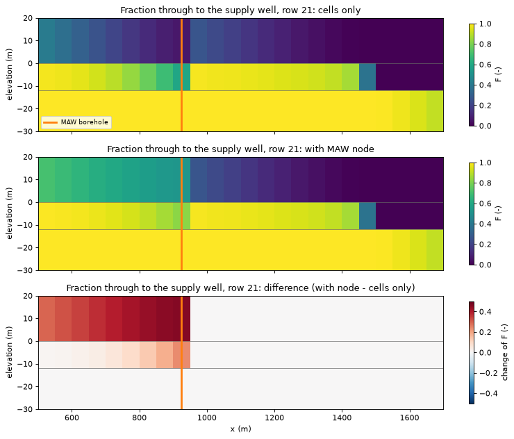
Without the node, the borehole is a sink in layers 1 and 2, so the water it takes there looks lost: only 6 % of the water in the MAW’s layer-1 cell reaches the supply well. With the node, that rises to 52 %. The change reaches up-gradient through layer 1 west of the borehole, whose water flows towards it, and is smaller in the aquitard. Layer 3 is unchanged, because the MAW’s inflow there was already traced to the well. The MAW pumps only 10 m³/d, less than half of the water that flows through its borehole. A long-screened well that pumps little can short-circuit an aquitard in this way. Water from a shallow aquifer, with whatever it carries, can then reach a deep supply aquifer.
5. A split model gives the same answer#
Large models are sometimes split into several GWF models joined by GWF-GWF exchanges, for parallel runs or different grids. gwsource reads all models of a simulation into one global graph: the cells of every model, numbered model by model, with each exchange flow as an edge between the two cells it joins.
To show that nothing is lost, we split the quickstart model of tutorial 01 into three models with FloPy’s Mf6Splitter (through hbd.split_model, which also switches on SAVE_FLOWS in every exchange). The west half becomes one model, and the east half becomes a north-east and a south-east quarter. The supply well and the stream cross into different models.
single = hbd.build_quickstart(WORK / "single", MF6)
spec = single.spec
labels = np.zeros((spec.nrow, spec.ncol), dtype=int)  # one model number per cell
labels[:SPLIT_ROW, SPLIT_COL:] = 1
labels[SPLIT_ROW:, SPLIT_COL:] = 2
splitter = hbd.split_model(single, labels, WORK / "split", MF6)

exchange_file = sorted((WORK / "split").glob("*.gwfgwf"))[0]
options = exchange_file.read_text(encoding="utf-8").split("END options")[0]
print(exchange_file.name)
print("\n".join(line for line in options.splitlines() if line.strip() and not line.startswith("#")))
sim_quickstart_0_quickstart_1.gwfgwf
BEGIN options
  auxiliary  ANGLDEGX  CDIST
  SAVE_FLOWS
single_step = gs.read_step(single.ws, boundnames=True)
ax = hbd.plot_cells(single.grb_file, single_step, labels.ravel().astype(float), cmap="Pastel2", vmin=0, vmax=7,
                    title="Split layout: three GWF models", colorbar=False)
helpers.model_boundaries(ax, labels, spec.delr, spec.delc)
for number, (x, y) in enumerate(((500.0, 1000.0), (1500.0, 1500.0), (1500.0, 500.0))):
    ax.text(x, y, f"quickstart_{number}", ha="center", fontsize=11, weight="bold")
plt.show()
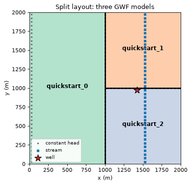
gs.open_simulation (or gs.read_network for one step) reads every GWF model listed in mfsim.nam. It checks that every exchange between two models it reads has SAVE_FLOWS, since the exchange flows are in the budget files only then. Term names get a <model>/ prefix. Selectors match with or without it, so boundnames=[WELL] and package="RCH" work across models.
split = gs.read_network(WORK / "split", boundnames=True)
for block in split.blocks:
    print(f"{block.label}: nodes {block.offset}..{block.offset + block.n - 1}, grid {block.grid_shape}")
print("terms:", ", ".join(split.package_names))
print("exchanges read as edges:", ", ".join(split.notes["exchanges"]))

back_single = gs.backward(single_step, {WELL: gs.select(single_step, boundnames=[WELL])})
back_split = gs.backward(split, {WELL: gs.select(split, boundnames=[WELL])})

rows = {}
for output in ("fraction_through", "volume_through", "volume_from"):
    reference = getattr(back_single, output)[WELL]
    mapped = hbd.map_back(splitter, split, getattr(back_split, output)[WELL])  # to the original cells
    largest = np.abs(mapped - reference).max()
    rows[output] = {"max |split - single|": largest, "max |single|": np.abs(reference).max(),
                    "relative": largest / np.abs(reference).max()}
display(pd.DataFrame(rows).T)
F_split = hbd.map_back(splitter, split, back_split.fraction_through[WELL])
assert np.abs(F_split - back_single.fraction_through[WELL]).max() < 1e-8
quickstart_0: nodes 0..799, grid (1, 40, 20)
quickstart_1: nodes 800..1199, grid (1, 20, 20)
quickstart_2: nodes 1200..1599, grid (1, 20, 20)
terms: quickstart_0/RCH, quickstart_0/CHD, quickstart_1/RCH, quickstart_1/SFR, quickstart_2/WEL, quickstart_2/RCH, quickstart_2/SFR
exchanges read as edges: GWF-GWF_1, GWF-GWF_2, GWF-GWF_3
| max |split - single| | max |single| | relative | |
|---|---|---|---|
| fraction_through | 1.350146e-09 | 1.000000 | 1.350146e-09 |
| volume_through | 1.093595e-08 | 800.000000 | 1.366994e-11 |
| volume_from | 1.848412e-08 | 51.049736 | 3.620805e-10 |
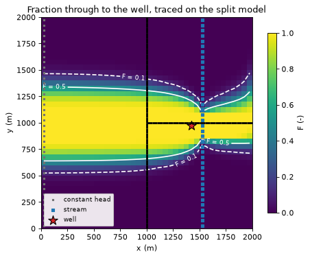
hbd.map_back uses the splitter’s node map to put each model’s values back on the original grid. The largest difference in \(F\) is \(1.4 \times 10^{-9}\). MF6 solves the split simulation as a different linear system. Its heads and flows are therefore not bit-for-bit those of the single model, although both are solved to the same tolerance. The splitter also cuts the stream in two and joins the halves with a mover between the models. The stream’s stage depends on its flow, so the two simulations differ a little more than for a model without a stream. The fractions agree to about \(10^{-9}\). The other outputs agree to \(4 \times 10^{-10}\) or better, relative to their largest value. The trace does not need the mover between the models: on the cells alone, the stream reaches are source and sink terms of their cells. The test suite checks every output, forward and backward, including travel times, on DIS, DISV and transient splits.
ax = hbd.plot_cells(single.grb_file, single_step, F_split, cmap="viridis", vmin=0.0, vmax=1.0,
                    title="Fraction through to the well, traced on the split model", label="F (-)")
hbd.add_contours(ax, single.grb_file, single_step, F_split, (0.1, 0.5), colors="w", linestyles=["--", "-"])
helpers.model_boundaries(ax, labels, spec.delr, spec.delc)
plt.show()
display(hbd.volume_from_table(back_split, WELL).round({"volume_from": 1, "share": 3}))
| volume_from | share | |
|---|---|---|
| source | ||
| quickstart_0/RCH | 327.9 | 0.410 |
| quickstart_2/RCH | 123.3 | 0.154 |
| quickstart_0/CHD | 122.4 | 0.153 |
| quickstart_1/RCH | 114.7 | 0.143 |
| quickstart_2/SFR | 79.9 | 0.100 |
| quickstart_1/SFR | 31.8 | 0.040 |
The capture zone crosses two model boundaries without a seam, and it matches tutorial 01. Because the source terms keep their model prefix, the volume-from table also splits the well’s water by model. The well in the south-east model takes most of its recharge from the west model, and its stream water from both eastern models.
One model on its own#
Read alone with gs.read_step(ws, model=...), a model of the split simulation treats its exchanges as boundary terms (GWF-GWF), the same way the cells-only trace treated the stream. Water that crossed from a neighbouring model has no history:
alone = gs.read_step(WORK / "split", model="quickstart_2", boundnames=True)
back_alone = gs.backward(alone, {WELL: gs.select(alone, boundnames=[WELL])})
display(hbd.volume_from_table(back_alone, WELL).round({"volume_from": 1, "share": 3}))
| volume_from | share | |
|---|---|---|
| source | ||
| GWF-GWF_3 | 357.9 | 0.447 |
| GWF-GWF_2 | 238.9 | 0.299 |
| RCH | 123.3 | 0.154 |
| SFR | 79.9 | 0.100 |
print(f"notebook runtime: {time.perf_counter() - T_START:.0f} s")
notebook runtime: 1 s
6. What MODFLOW 6 must save, and current limits#
To trace through |
MF6 option |
If it is missing |
|---|---|---|
any model (as in every tutorial) |
|
– |
GWF-GWF exchanges |
|
|
SFR, LAK, MAW or UZF nodes |
|
|
MVR transfers (in a model with package nodes) |
|
|
Package nodes are optional: without package_nodes, open_simulation gives the cells-only results of section 2 exactly.
Current limitations:
Movers between models (the simulation-level MVE package) are not read. Movers inside one model are.
A mover transfer becomes an edge only if the receiving package has nodes and the provider’s
TO-MVRrecord is in the graph. Otherwise it stays a sink on the provider and a source on the receiver, as in section 2.Package nodes take their water volume (for travel times and transient tracking) from the
VOLUMEof the package’sSTORAGErecord. Flux outputs (per unit area) are not defined on package nodes (NaN).Tested on MF6 models: SFR + MVR, MAW across layers, LAK with outlets, UZF with rejected infiltration moved to a lake, and splits of DIS, DISV and transient models. Covered only by hand-built tests: multi-layer UZF cell-to-cell flow, MAW flowing wells, and LAK or MAW as mover providers.
The MF6 PRT particle helper of tutorial 06 works on single-model steps without package nodes only.
Per-model output:
gs.result_view/gs.model_viewcut a network result down to one model’s cells for the single-model exports.gs.export.save_networkwrites one npz per model, a CSV of the package nodes and a GeoPackage with a point layer for them.
Key points#
Water that leaves the cells and comes back (through a stream, a mover, a well bore or another model) breaks a cells-only trace into an opaque sink and an opaque source.
gs.open_simulation(ws, package_nodes=(...))adds one node per SFR reach, lake, MAW well or UZF cell, turns the package exchange records and MVR transfers into edges, and reads every GWF model of the simulation with exchanges as edges. Everything downstream (backward, forward, metrics, diagnostics, travel time, transient tracking) works on the larger graph unchanged.Stream and mover: with SFR nodes, the area that drains to the stream above the well and the drained area joined the well’s catchment, and the “SFR” source split into recharge and west-edge water, part of which travelled drain → mover → stream → aquifer.
MAW: the borehole is a fully mixed node, so a weakly pumped well screened across an aquitard shows up as a short circuit that feeds the deeper supply well.
A split simulation gives the single model’s fractions to about \(10^{-9}\). Read alone, a model’s exchanges are boundary terms.
These features need
SAVE_FLOWSon the exchanges andBUDGET FILEOUTon the advanced packages and MVR.
Next#
08 · Transient tracking: carry tagged water through storage from step to step, forward and backward, and compare with MF6 GWT.