11 · Numerical dispersion: how wide is the edge of a capture zone, and how does it change with the grid?

Full mixing assumes that the water entering a cell leaves it through all its outflow faces, in proportion to their flows. Near the edge of a capture zone, every cell therefore splits the water it receives into a part that reaches the well and a part that does not. The edge of the zone is smeared over a band of cells with intermediate fractions. This spreading comes from the grid, not from the aquifer. We call it numerical dispersion.

This tutorial measures that band on two test problems with references that do not mix:

• Problem A, uniform regional flow and a well, against the analytical capture zone of Javandel and Tsang (1986);

• Problem B, a recharge-fed model with a river, against flow-weighted MF6 PRT particles on a fine grid.

You will:

1. build problem A on square (DIS) and Voronoi (DISV) cells of 200 to 12.5 m, with the flow along the grid rows and at 30° to them;

2. measure how wide the edge is and how fast it narrows as the cells get smaller;

3. build problem B and its particle reference;

4. repeat the measurements on problem B, west of the river;

5. turn the grid of the tutorial aquifer by 45° to the flow and see how the edge widens;

6. check that the well’s shares by source and its mean travel time hardly depend on the mixing;

7. collect the numbers in one table.

Terms used. \(F\) is the fraction through (tutorial 01): the share of a cell’s water that reaches the well. The band is the area where \(0.1 < F < 0.9\). Its width is that area divided by the length of the reference zone edge. It is the mean distance between the \(F = 0.1\) and \(F = 0.9\) contours across the edge. \(h\) is the cell size, and for Voronoi grids the square root of the mean cell area. Face routing is an experimental 2D option (gwsource.experimental.face_routing, after Chowdhury 2016) that passes water from each inflow face to the outflow faces it reaches, instead of mixing it over the whole cell.

Runtime: about 1 minute (the last code cell prints the measured time). The PRT run on the finest grid of problem B takes about 25 s of it. Prerequisites: tutorials 01 and 04; bin/mf6 and bin/triangle (downloaded by scripts/setup_env.py); the Python package vorflow for section 5 (in environment.yml).

Settings

All settings live in this first cell. Workspaces go to tutorials/_work/11_numerical_dispersion/ (git-ignored, recreated on every run). The shared helpers are in herebedragons.py. The test problems, the references and the edge metrics of this tutorial are in helpers.py, next to this notebook.

Every per-cell field is sampled on one raster of 2.5 m points shared by all grids, so different grids are compared on the same points. The comparison leaves out a band along the model boundary: 200 m wide in problem A, where the perimeter cells hold fixed heads, and 25 m in problem B.

import sys
import time
from pathlib import Path

import matplotlib.pyplot as plt
import numpy as np
import pandas as pd

sys.path.insert(0, str(Path.cwd().parent))  # tutorials/ holds the shared helpers
sys.path.insert(0, str(Path.cwd()))  # this folder holds helpers.py
import herebedragons as hbd  # noqa: E402
import helpers  # noqa: E402  (this tutorial's test problems, references and metrics)

import gwsource as gs  # noqa: E402

START = time.perf_counter()  # the notebook prints its run time at the end
WORK = hbd.work_dir("11_numerical_dispersion", clean=True)  # tutorials/_work/... (git-ignored)
MF6 = hbd.mf6_exe()  # <repo>/bin/mf6
TRIANGLE = hbd.exe_path("triangle")  # <repo>/bin/triangle, meshes the Voronoi grids
SIZES_A = (200.0, 100.0, 50.0, 25.0, 12.5)  # m, cell sizes of problem A
SIZES_B = (100.0, 50.0, 25.0, 12.5)  # m, cell sizes of problem B (PRT on the finest is the reference)
ANGLES = (0.0, 30.0)  # degrees between the regional flow and the grid rows (problem A)
KINDS = ("DIS", "DISV")  # square cells and Voronoi cells (Triangle maximum area h^2)
RASTER = 2.5  # m, spacing of the shared comparison raster
MARGIN_A, MARGIN_B = 200.0, 25.0  # m, band along the model boundary left out of the comparison
RIVER_GAP = 50.0  # m, problem B is compared west of x = river - RIVER_GAP
POROSITY = 0.3  # for travel times and PRT
PRT_SUBDIVISIONS = 2  # 16 release points per DIS cell
MAP_H = 50.0  # m, cell size of the maps
FINE = 50.0  # m, "cells of 50 m or less"
STYLES = {  # (grid, method): line style of the convergence plots
    ("DIS", "full mixing"): {"color": "tab:blue", "marker": "o"},
    ("DIS", "face routing"): {"color": "tab:orange", "marker": "s"},
    ("DISV", "full mixing"): {"color": "tab:green", "marker": "^"},
    ("DIS", "cell-averaged exact"): {"color": "0.4", "marker": "x"},
    ("DIS", "PRT"): {"color": "0.4", "marker": "x"},
}
# section 5: the tutorial aquifer of tutorials 01 and 04 on three grids
WELL = "supply_well"  # boundname of its well
ROTATED_SIDE = 100.0 / 3.0 * np.sqrt(2.0)  # m, squares turned 45 degrees (as in tutorial 04)
VORONOI_SIZES = {"background": 25.0, "well_size": 10.0, "river_size": 12.5}  # m, vorflow mesh sizes
TRANSECT_X = 500.0  # m, north-south line on which the width of the edge is measured

plt.rcParams.update({"figure.dpi": 80})
vorflow = hbd.require_vorflow()  # optional dependency: only section 5 needs it
print(f"gwsource {gs.__version__}, vorflow {vorflow.__version__}")

gwsource 0.0.1, vorflow 0.3.0

1. Problem A: uniform flow and a well

Problem A is a confined aquifer, 2 km × 2 km, with a transmissivity \(T\) of 500 m²/d and a regional hydraulic gradient \(i\) of 0.002. The regional discharge per unit width is \(U = T i\) = 1 m²/d. One well pumps \(Q\) = 500 m³/d. The heads of all perimeter cells are fixed to the analytical head of uniform flow plus a well,

\[h = h_0 - i\,s + \frac{Q}{4\pi T}\ln r^2,\]

where \(s\) is the distance along the regional flow and \(r\) the distance from the well. The flow inside the domain then approaches uniform flow plus a well. Its capture zone is known exactly (Javandel and Tsang 1986). Far upstream the zone is \(Q/U\) = 500 m wide. Its edge, the dividing streamline, passes through a stagnation point \(Q/(2\pi U)\) = 80 m downstream of the well.

The cell below builds the problem on five cell sizes, on DIS and Voronoi DISV grids, with the regional flow along the grid rows (0°) and at 30° to them. That makes 20 models. On each it computes three fields:

• full mixing, the backward trace of tutorial 01;

• face routing, on DIS only;

• the cell-averaged exact zone: the analytical zone averaged over each cell. It is the best a field with one value per cell can do, and sets the floor of the band width.

The flux-weighted mean travel time of the water reaching the well is \(\sum_i n\,b\,A_i F_i / Q\) under full mixing (tutorial 06), with \(n\) the porosity and \(b\) the thickness. The analytical value is \(n\,b\) times the zone area, over \(Q\). So the relative error of the travel time is \(\sum_i A_i F_i\) over the analytical zone area, minus 1. The cell computes it for every field.

specs_a = {angle: helpers.ProblemA(angle_deg=angle) for angle in ANGLES}
spec = specs_a[0.0]
print(f"U = {spec.regional_discharge:g} m2/d, zone width Q/U = {spec.rate / spec.regional_discharge:.0f} m, "
      f"stagnation point Q/(2 pi U) = {spec.rate / (2 * np.pi * spec.regional_discharge):.1f} m downstream")

t0 = time.perf_counter()
rasters_a, runs_a, rows = {}, {}, []
for angle, spec in specs_a.items():
    raster = helpers.make_raster(spec.lx, spec.ly, RASTER, MARGIN_A)
    raster.set_reference(helpers.capture_zone_mask(raster.xr, raster.yr, spec))
    rasters_a[angle] = raster
    zone_area = raster.ref.sum() * raster.pixel  # analytical zone area in the whole domain
    for kind in KINDS:
        for h in SIZES_A:
            run = helpers.problem_a_run(WORK / f"a{angle:g}_{kind}_{h:g}", MF6, TRIANGLE, spec, kind, h, raster)
            runs_a[(angle, kind, h)] = run
            for row in helpers.metrics_rows({"angle": angle, "kind": kind, "h": h}, run, raster):
                F = run["fields"][row["method"]]
                row["travel_time_err"] = float(F @ run["step"].area / zone_area - 1.0)
                rows.append(row)
table_a = pd.DataFrame(rows)
cells = table_a.drop_duplicates(["angle", "kind", "h"])
print(f"{len(cells)} models of {cells['cells'].min()} to {cells['cells'].max()} cells, "
      f"traced and compared in {time.perf_counter() - t0:.0f} s")
display(cells[cells["angle"] == 0.0].pivot(index="h", columns="kind", values=["cells", "mean_h"])
        .sort_index(ascending=False).round(0))

U = 1 m2/d, zone width Q/U = 500 m, stagnation point Q/(2 pi U) = 79.6 m downstream

20 models of 91 to 25600 cells, traced and compared in 11 s

	cells		mean_h
kind	DIS	DISV	DIS	DISV
h
200.0	100.0	91.0	200.0	210.0
100.0	400.0	349.0	100.0	107.0
50.0	1600.0	1322.0	50.0	55.0
25.0	6400.0	5207.0	25.0	28.0
12.5	25600.0	20450.0	12.0	14.0

The Voronoi grids made with Triangle at a maximum triangle area of \(h^2\) have mean cell sizes of 210, 107, 55, 28 and 14 m. They are a little coarser than the DIS grid of the same \(h\). The plots below use the mean cell size.

The maps show the four fields on 50 m cells, with the flow at 30° to the rows. The dashed line is the analytical edge.

angle = 30.0
spec = specs_a[angle]
x_edge, y_edge = helpers.divide_line(spec)
panels = [("DIS", "cell-averaged exact"), ("DIS", "full mixing"), ("DIS", "face routing"), ("DISV", "full mixing")]
fig, axes = plt.subplots(1, 4, figsize=(19.0, 4.6))
for ax, (kind, method) in zip(axes, panels):
    run = runs_a[(angle, kind, MAP_H)]
    helpers.plot_field(ax, run["model"], run["step"], run["fields"][method], f"{kind} {MAP_H:g} m: {method}",
                       (spec.well_x, spec.well_y))
    ax.plot(x_edge, y_edge, "w--", lw=1.2)
    ax.set_xlim(0.0, spec.lx)
    ax.set_ylim(0.0, spec.ly)
fig.colorbar(axes[-1].collections[0], ax=axes, shrink=0.85, label="F (-)")
fig.suptitle(f"Problem A, regional flow at {angle:g} degrees to the rows: fraction of the water in each cell "
             "that reaches the well")
plt.show()

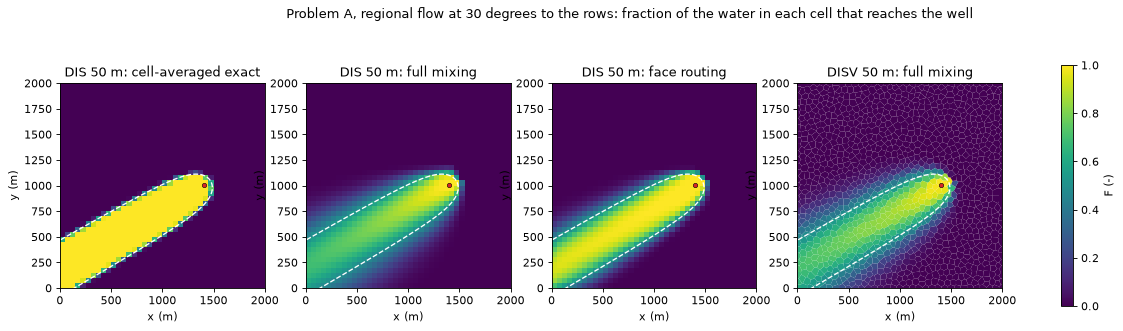
The cell-averaged exact zone (left) has a band of about one cell: only the cells that the edge crosses hold intermediate values. Full mixing spreads the edge over several cells on each side. The spreading grows with the distance travelled along the edge, so the band is widest far upstream and narrowest near the well. Face routing gives a narrower band. The Voronoi band is about as wide as the DIS band.

2. How the edge narrows with the cell size

The table gives the metrics for 50 m and 12.5 m cells. Area errors are relative to the analytical zone. Missed is the share of the analytical zone where \(F\) is not above the threshold.

COLUMNS = {"area_err_0.01": "area err F>0.01", "area_err_0.1": "area err F>0.1", "area_err_0.5": "area err F>0.5",
           "jaccard_0.5": "Jaccard F>0.5", "missed_0.1": "missed F>0.1", "missed_0.5": "missed F>0.5",
           "band_width": "band width (m)", "band_cells": "band (cells)", "travel_time_err": "travel time err"}


def show(table: pd.DataFrame, index: list[str], columns: dict) -> None:
    # display selected metrics, three decimals (band width in metres, one decimal)
    out = table.set_index(index)[list(columns)].rename(columns=columns)
    display(out.style.format("{:.3f}").format("{:.0f}", subset=["band width (m)"])
            .format("{:.1f}", subset=["band (cells)"]))


selected = table_a[table_a["h"].isin([50.0, 12.5])].sort_values(["angle", "h", "kind"], ascending=[True, False, True])
show(selected, ["angle", "kind", "h", "method"], COLUMNS)

				area err F>0.01	area err F>0.1	area err F>0.5	Jaccard F>0.5	missed F>0.1	missed F>0.5	band width (m)	band (cells)	travel time err
angle	kind	h	method
0.000000	DIS	50.000000	full mixing	1.285	0.670	0.016	0.887	0.000	0.052	214	4.3	0.037
			face routing	0.794	0.431	0.021	0.891	0.000	0.048	156	3.1	0.027
			cell-averaged exact	0.135	0.121	0.011	0.922	0.001	0.035	44	0.9	0.000
	DISV	50.000000	full mixing	1.596	0.900	0.027	0.905	0.000	0.037	324	5.9	0.036
			cell-averaged exact	0.183	0.117	-0.006	0.937	0.003	0.035	41	0.7	0.000
	DIS	12.500000	full mixing	0.561	0.299	0.000	0.980	0.000	0.010	105	8.4	0.007
			face routing	0.355	0.194	0.002	0.980	0.000	0.009	69	5.5	0.005
			cell-averaged exact	0.028	0.026	-0.000	0.984	0.000	0.008	10	0.8	0.000
	DISV	12.500000	full mixing	0.736	0.399	-0.007	0.967	0.000	0.020	147	10.5	-0.000
			cell-averaged exact	0.038	0.028	-0.000	0.982	0.001	0.009	11	0.8	-0.000
30.000000	DIS	50.000000	full mixing	1.013	0.674	0.045	0.922	0.000	0.019	304	6.1	-0.025
			face routing	0.665	0.414	0.032	0.929	0.000	0.021	167	3.3	0.004
			cell-averaged exact	0.138	0.092	-0.010	0.945	0.002	0.033	35	0.7	0.000
	DISV	50.000000	full mixing	1.180	0.706	0.045	0.929	0.000	0.015	317	5.8	-0.015
			cell-averaged exact	0.148	0.083	0.003	0.941	0.003	0.029	37	0.7	0.000
	DIS	12.500000	full mixing	0.563	0.341	0.009	0.984	0.000	0.004	148	11.8	-0.012
			face routing	0.326	0.189	0.005	0.986	0.000	0.005	77	6.1	-0.002
			cell-averaged exact	0.030	0.021	0.001	0.987	0.001	0.006	8	0.7	0.000
	DISV	12.500000	full mixing	0.585	0.338	-0.002	0.979	0.000	0.012	147	10.5	-0.017
			cell-averaged exact	0.035	0.025	0.002	0.984	0.001	0.007	10	0.7	0.000

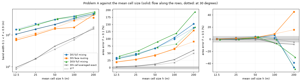
• The F > 0.5 area is close to the analytical area: within 5 % at 50 m and within 1 % at 12.5 m, for every method.

• The F > 0.1 area never misses more than 0.01 % of the analytical zone, but it is much too large: by 67 to 90 % at 50 m and by 30 to 40 % at 12.5 m under full mixing.

• The band of full mixing is 214 m (0°) and 304 m (30°) wide at 50 m. At 12.5 m it is 105 m and 148 m, that is 8 to 12 cells.

The plots show the whole series. Solid lines: flow along the rows. Dotted: flow at 30°. The dashed guide falls as \(h^{0.5}\). The grey band is ±5 %.

series_a = []
for angle, line in ((0.0, "-"), (30.0, ":")):
    for (kind, method), style in STYLES.items():
        if method != "PRT":
            label = f"{kind} {method}" if angle == 0.0 else None
            series_a.append((label, {"angle": angle, "kind": kind, "method": method}, {**style, "ls": line}))
fig, axes = plt.subplots(1, 3, figsize=(16.0, 4.4))
helpers.plot_convergence(axes, table_a, series_a, guide_h=(12.5, 200.0))
axes[0].legend(fontsize=8)
fig.suptitle("Problem A against the mean cell size (solid: flow along the rows, dotted: at 30 degrees)")
fig.tight_layout()
plt.show()

rates_a = helpers.rates_table(table_a, ["angle", "kind", "method"])
print("convergence rates: slope of log(metric) against log(mean cell size), five grids")
display(rates_a.round(2))

convergence rates: slope of log(metric) against log(mean cell size), five grids

			band_width	area_err_0.1
angle	kind	method
0.0	DIS	cell-averaged exact	1.03	1.15
		face routing	0.60	0.66
		full mixing	0.54	0.59
	DISV	cell-averaged exact	1.04	1.08
		full mixing	0.47	0.57
30.0	DIS	cell-averaged exact	1.07	1.09
		face routing	0.57	0.58
		full mixing	0.41	0.51
	DISV	cell-averaged exact	1.06	1.03
		full mixing	0.42	0.50

The cell-averaged exact zone converges at first order: its band stays at about 0.7 to 0.9 cells at every size. Full mixing converges at about half order. Its band narrows as about \(h^{0.5}\), with fitted rates of 0.41 to 0.54. In cells, the band therefore grows as the grid gets finer, from 2 cells at 200 m to 12 cells at 12.5 m. The spreading behaves like a diffusion with a coefficient proportional to the cell size: the band grows with the square root of \(h\) times the distance travelled along the edge.

Face routing narrows the band but keeps the half-order rate (0.57 and 0.60). It still mixes the water across each cell face. The Voronoi grids spread the edge no less than the squares. With the flow at 30°, their band equals that of DIS (147 m against 148 m at about 13 m). With the flow along the rows, it is wider (147 m against 105 m).

3. Problem B: a recharge-fed zone and its particle reference

Problem B has the physics of one of the package’s test models, without its inactive cells. It is one unconfined layer, 1.5 km × 1 km, with recharge of 1 mm/d, a river along \(x\) = 1128 m, a constant head on the west edge and a well pumping 800 m³/d. The well and the river sit at points that are inside cells for every cell size. The river conductance is given per metre of river, so it does not change with the grid.

Here the reference is MF6 PRT, through gwsource.prt.track_particles (tutorial 06). On every DIS grid, 16 particles per cell are released in every cell with \(F > 0\) and weighted by the cell’s recharge. The run on the finest grid, 12.5 m, is the reference. It is compared with the fraction of each cell’s recharge that reaches the well. Under full mixing that fraction is \(F\) of the cell. Under face routing it is the fraction of the recharge, which enters through the top face.

East of the river all water passes the gaining river, which is a weak sink. The PRT helper, too, treats weak sinks by full mixing: it reduces the weight of a particle by the share that the river removes from each cell it passes. The areas are therefore compared west of the river only, 50 m or more from it, where no method mixes at a weak sink.

spec_b = helpers.ProblemB()
raster_b = helpers.make_raster(spec_b.lx, spec_b.ly, RASTER, MARGIN_B)
raster_b.window &= raster_b.xr < spec_b.riv_x - RIVER_GAP  # west of the river: no weak sinks on the way
runs_b = {}
for kind in KINDS:
    for h in SIZES_B:
        t0 = time.perf_counter()
        run = helpers.problem_b_run(WORK / f"b_{kind}_{h:g}", MF6, TRIANGLE, spec_b, kind, h, POROSITY,
                                    PRT_SUBDIVISIONS)
        run["index"] = helpers.raster_cells(run["model"].modelgrid, raster_b)
        run["seconds"] = time.perf_counter() - t0
        runs_b[(kind, h)] = run
reference = runs_b[("DIS", min(SIZES_B))]
raster_b.set_reference(reference["fields"]["PRT"][reference["index"]])
prt = reference["prt"]
print(f"reference: PRT on DIS {min(SIZES_B):g} m, {reference['model'].n_cells} cells, {prt['n_particles']:,} particles; "
      f"captured flow {prt['captured_flow']:.2f} m3/d of {reference['well_inflow']:.2f} m3/d pumped")
display(pd.DataFrame({key: {"cells": run["model"].n_cells, "mean h (m)": run["model"].mean_cell_size,
                            "seconds": run["seconds"]} for key, run in runs_b.items()}).T.round(1))

rows = []
for (kind, h), run in runs_b.items():
    for row in helpers.metrics_rows({"kind": kind, "h": h}, run, raster_b):
        row["mean_time"] = run["mean_time"][row["method"]]
        row["share_RIV"] = run["shares"][row["method"]]["RIV"]
        rows.append(row)
table_b = pd.DataFrame(rows)

reference: PRT on DIS 12.5 m, 9600 cells, 93,856 particles; captured flow 800.86 m3/d of 800.00 m3/d pumped

		cells	mean h (m)	seconds
DIS	100.0	150.0	100.0	0.2
	50.0	600.0	50.0	0.5
	25.0	2400.0	25.0	2.4
	12.5	9600.0	12.5	16.3
DISV	100.0	140.0	103.5	0.1
	50.0	525.0	53.5	0.1
	25.0	1972.0	27.6	0.4
	12.5	7721.0	13.9	1.3

The 93,856 particles capture 800.9 m³/d, 0.1 % more than the pumping. The difference comes from placing a finite number of release points. The run on 12.5 m cells takes most of the time of this cell.

The maps show the PRT reference on 12.5 m cells and the three methods on 50 m cells. The dashed line is the reference edge, the PRT \(F = 0.5\) contour. The grey line is the river. The comparison window ends at the dotted line.

panels = [(("DIS", 12.5), "PRT"), (("DIS", MAP_H), "full mixing"), (("DIS", MAP_H), "face routing"),
          (("DISV", MAP_H), "full mixing")]
xr, yr, ref = raster_b.xr, raster_b.yr, np.ma.masked_where(~raster_b.window, raster_b.ref)
fig, axes = plt.subplots(1, 4, figsize=(19.0, 3.9))
for ax, (key, method) in zip(axes, panels):
    run = runs_b[key]
    helpers.plot_field(ax, run["model"], run["step"], run["fields"][method], f"{key[0]} {key[1]:g} m: {method}",
                       (spec_b.well_x, spec_b.well_y))
    ax.contour(xr, yr, ref, levels=[0.5], colors="w", linestyles="--", linewidths=1.2)
    ax.axvline(spec_b.riv_x, color="0.6", lw=2.0)
    ax.axvline(spec_b.riv_x - RIVER_GAP, color="w", ls=":", lw=1.0)
fig.colorbar(axes[-1].collections[0], ax=axes, shrink=0.85, label="F (-)")
fig.suptitle("Problem B: fraction of each cell's recharge that reaches the well")
plt.show()

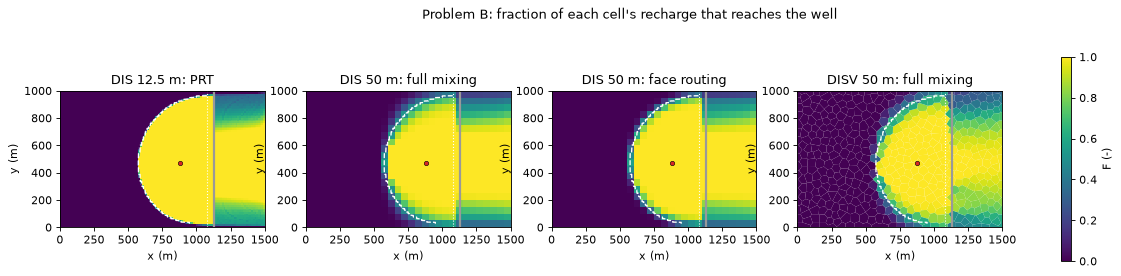
The well captures the recharge of an area that reaches back to the west edge. On 50 m cells, full mixing smears its edge over about two cells, face routing over about one. East of the river every method gives partial fractions, because the gaining river takes part of the water of every cell it drains.

4. Problem B against the cell size

The area errors are now relative to the PRT reference zone, \(F_\mathrm{PRT} \ge 0.5\) on 12.5 m cells. The reference compared with itself has non-zero errors at the low thresholds, because its fractions are graded where the edge crosses a cell. Its F > 0.5 area is 0.5 % smaller than the reference area, because a few of its cells hold exactly 0.5: they are in the reference zone (\(\ge 0.5\)) but not in the F > 0.5 area.

show(table_b.sort_values(["kind", "h"], ascending=[True, False]), ["kind", "h", "method"],
     {**{k: v for k, v in COLUMNS.items() if k != "travel_time_err"}, "mean_time": "mean travel time (d)"})

			area err F>0.01	area err F>0.1	area err F>0.5	Jaccard F>0.5	missed F>0.1	missed F>0.5	band width (m)	band (cells)	mean travel time (d)
kind	h	method
DIS	100.000000	full mixing	0.403	0.278	-0.005	0.910	0.000	0.050	122	1.2	9940.152
		face routing	0.265	0.212	-0.025	0.905	0.000	0.062	92	0.9	9990.978
		PRT	0.166	0.166	-0.040	0.895	0.004	0.074	76	0.8	9785.998
	50.000000	full mixing	0.248	0.163	-0.017	0.948	0.000	0.035	82	1.6	9667.966
		face routing	0.156	0.090	-0.040	0.941	0.000	0.049	54	1.1	9686.475
		PRT	0.067	0.061	-0.040	0.941	0.003	0.049	33	0.7	9647.579
	25.000000	full mixing	0.168	0.102	-0.013	0.974	0.000	0.020	58	2.3	9685.818
		face routing	0.089	0.051	-0.015	0.976	0.000	0.019	33	1.3	9693.514
		PRT	0.028	0.020	-0.020	0.973	0.002	0.023	18	0.7	9690.571
	12.500000	full mixing	0.143	0.085	-0.001	0.997	0.000	0.002	41	3.3	9730.738
		face routing	0.077	0.045	-0.002	0.998	0.000	0.002	22	1.8	9734.529
		PRT	0.021	0.018	-0.005	0.995	0.000	0.005	8	0.7	9750.363
DISV	100.000000	full mixing	0.261	0.198	0.003	0.935	0.001	0.032	115	1.1	8758.652
	50.000000	full mixing	0.250	0.151	0.007	0.951	0.000	0.021	79	1.5	9554.536
	25.000000	full mixing	0.178	0.105	-0.007	0.965	0.000	0.021	56	2.0	9562.578
	12.500000	full mixing	0.161	0.101	0.018	0.976	0.000	0.003	42	3.0	9787.027

series_b = [(f"{kind} {method}", {"kind": kind, "method": method}, style)
            for (kind, method), style in STYLES.items() if method != "cell-averaged exact"]
fig, axes = plt.subplots(1, 3, figsize=(16.0, 4.4))
helpers.plot_convergence(axes, table_b, series_b, guide_h=(12.5, 100.0))
axes[0].legend(fontsize=8)
fig.suptitle("Problem B against the mean cell size, west of the river (grey: PRT on each DIS grid)")
fig.tight_layout()
plt.show()

rates_b = helpers.rates_table(table_b, ["kind", "method"])
print("convergence rates: slope of log(metric) against log(mean cell size), four grids")
display(rates_b.round(2))

convergence rates: slope of log(metric) against log(mean cell size), four grids

		band_width	area_err_0.1
kind	method
DIS	PRT	1.05	1.13
	face routing	0.68	0.75
	full mixing	0.53	0.58
DISV	full mixing	0.51	0.36

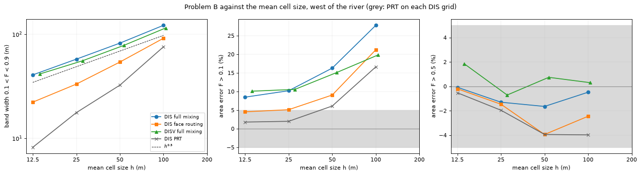
The picture is the one of problem A, with smaller numbers:

• The band of full mixing is 1.1 to 3.3 cells wide. It narrows at a rate of 0.53 on DIS and 0.51 on DISV. PRT on each coarser grid sets the floor of about 0.7 cells.

• The F > 0.5 area is within 4 % of the reference for every method at 50 m or less (2 % under full mixing).

• The F > 0.1 area of full mixing misses at most 0.13 % of the reference zone, on the coarsest Voronoi grid, and at most 0.02 % at 50 m or less. It is 8 to 16 % too large at 12.5 to 50 m, much less than in problem A. Here the zone edge is a recharge divide, close to where the water enters. In problem A it is a long streamline fed by lateral inflow, along which the spreading builds up.

How much of the extra spreading does face routing remove? The cell below compares the band widths in excess of the floor: the cell-averaged exact zone in problem A, and PRT on the same grid in problem B.

def removed(table: pd.DataFrame, keys: list[str], floor: str) -> pd.Series:
    # share of the band width in excess of the floor that face routing removes, per grid
    dis = table[table["kind"] == "DIS"].pivot_table(index=keys, columns="method", values="band_width")
    return 1.0 - (dis["face routing"] - dis[floor]) / (dis["full mixing"] - dis[floor])


excess = pd.concat({
    "problem A, 0 degrees": removed(table_a[table_a["angle"] == 0.0], ["h"], "cell-averaged exact"),
    "problem A, 30 degrees": removed(table_a[table_a["angle"] == 30.0], ["h"], "cell-averaged exact"),
    "problem B": removed(table_b, ["h"], "PRT"),
}, axis=1).sort_index(ascending=False)
print("share of the excess band width removed by face routing")
display(excess.round(2))

share of the excess band width removed by face routing

	problem A, 0 degrees	problem A, 30 degrees	problem B
h
200.0	0.14	0.38	NaN
100.0	0.63	0.33	0.66
50.0	0.34	0.51	0.57
25.0	0.38	0.54	0.61
12.5	0.38	0.51	0.57

Face routing removes 34 to 61 % of the excess band width at 50 m or less: 34 to 38 % with the flow along the rows, about half at 30° and 57 to 61 % in problem B. Its band at \(h\) is close to that of full mixing at \(h/2\) (0°) or \(h/4\) (30°). It does not change the rate.

5. The orientation of the grid

Section 2 showed that the band depends on the angle between the flow and the cell faces. Tutorial 04 tested this on the tutorial aquifer: the 2 km × 2 km unconfined aquifer of tutorial 01, with recharge, a west constant head, a stream (SFR) and a well pumping 800 m³/d. The cell below repeats that test on four grids:

• the regular DIS grid of 50 m cells, whose rows run along the flow;

• squares turned by 45° to the flow, 47.1 m wide, one centred on the well (hbd.build_rotated_squares);

• the Voronoi grid of tutorial 04, about 50 m away from the well and the stream;

• the same Voronoi grid with a background size of 25 m.

The width of the edge is measured along the north–south line \(x\) = 500 m, north of the well. Along that line, \(F\) is interpolated linearly between the cell centres. The width is the distance from where \(F\) falls to 0.5 to where it falls to 0.1.

t0 = time.perf_counter()
example = {
    "DIS, 50 m": hbd.build_quickstart(WORK / "example_dis", MF6),
    "squares turned 45 degrees, 47 m": hbd.build_rotated_squares(WORK / "example_rotated", MF6, side=ROTATED_SIDE),
    "DISV, 50 m": hbd.build_voronoi(WORK / "example_disv50", MF6),
    "DISV, 25 m": hbd.build_voronoi(WORK / "example_disv25", MF6, **VORONOI_SIZES),
}
y = np.arange(0.0, example["DIS, 50 m"].spec.ly, 1.0)  # m, points along the line x = TRANSECT_X
profiles, edge_rows = {}, {}
for label, run in example.items():
    step = gs.read_step(run.ws, boundnames=True)
    F = gs.backward(step, {WELL: gs.select(step, boundnames=[WELL])}).fraction_through[WELL]
    profiles[label] = hbd.transect_profile(gs.export.cell_centres(run.grb_file), F, TRANSECT_X, y)
    y_half, y_tenth, width = hbd.band_width_north(y, profiles[label], 0.1, 0.5)
    edge_rows[label] = {"cells": step.n_cells, "expected area (km2)": float(F @ step.area) / 1e6,
                        "y at F = 0.5 (m)": y_half, "y at F = 0.1 (m)": y_tenth, "edge width (m)": width}
edges = pd.DataFrame(edge_rows).T
print(f"four grids built and traced in {time.perf_counter() - t0:.0f} s")
display(edges.round({"cells": 0, "expected area (km2)": 3, "y at F = 0.5 (m)": 0, "y at F = 0.1 (m)": 0,
                     "edge width (m)": 0}))
width = edges["edge width (m)"]
print(f"turned squares / DIS: {width.iloc[1] / width.iloc[0]:.2f}; "
      f"DISV 25 m / DISV 50 m: {width.iloc[3] / width.iloc[2]:.2f} (square root of 0.5: {np.sqrt(0.5):.2f})")

fig, ax = plt.subplots(figsize=(8.0, 4.0))
for label in example:
    ax.plot(y, profiles[label], label=f"{label} ({width[label]:.0f} m)")
for level in (0.1, 0.5):
    ax.axhline(level, color="0.6", ls=":", lw=1.0)
ax.set_xlim(1200.0, 1700.0)
ax.set_ylim(0.0, 1.02)
ax.set_xlabel(f"y (m), along x = {TRANSECT_X:g} m")
ax.set_ylabel("F (-)")
ax.set_title("F north of the well (width of the edge from 0.5 to 0.1 in brackets)")
ax.legend(fontsize=8)
plt.show()

four grids built and traced in 4 s

	cells	expected area (km2)	y at F = 0.5 (m)	y at F = 0.1 (m)	edge width (m)
DIS, 50 m	1600.0	1.167	1332.0	1456.0	124.0
squares turned 45 degrees, 47 m	1921.0	1.167	1340.0	1554.0	214.0
DISV, 50 m	3241.0	1.171	1340.0	1527.0	187.0
DISV, 25 m	8256.0	1.170	1339.0	1465.0	126.0

turned squares / DIS: 1.73; DISV 25 m / DISV 50 m: 0.67 (square root of 0.5: 0.71)

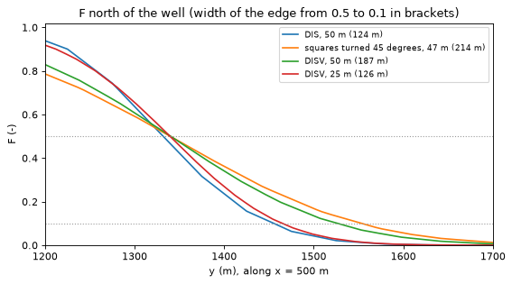
On the regular grid, \(F\) falls from 0.5 to 0.1 over 124 m. On the squares turned by 45°, the same band is 214 m wide, 1.7 times as wide, although these cells are a little smaller. Each turned square splits its water between two downstream faces, and every split moves some of the well’s share sideways. The 50 m Voronoi grid lies between the two, at 187 m. Its faces lie at many angles to the flow. Halving its background cell size narrows the edge to 126 m, 0.67 times as wide, close to the square-root rule of sections 2 and 4. The expected areas \(\sum_i F_i A_i\) of the four grids agree to within 0.5 %. The grid moves the edge, not the size of the zone.

6. The well’s water by source and its mean travel time

Spreading moves water across the edge in both directions. Do the integral outputs, which sum over the whole zone, depend on it? The first table gives the river’s share of the well water in problem B, under each method, on each grid. The second gives the mean travel time of all the water reaching the well, against the PRT reference, and the travel-time error of problem A against the analytical value.

shares = table_b.pivot_table(index=["kind", "h"], columns="method", values="share_RIV").sort_index(
    ascending=[True, False])[["full mixing", "face routing", "PRT"]]
print("problem B: share of the well water from the river (the rest is recharge)")
display(shares.round(4))
dis = shares.loc["DIS"]
spread = (dis.max(axis=1) - dis.min(axis=1)).max()
print(f"largest difference between the three methods on one DIS grid: {spread:.4f}")

time_b = table_b.pivot_table(index=["kind", "h"], columns="method", values="mean_time").sort_index(
    ascending=[True, False])[["full mixing", "face routing", "PRT"]]
time_b_err = time_b / prt["mean_time"] - 1.0
print(f"problem B: mean travel time relative to PRT on 12.5 m cells ({prt['mean_time']:.0f} d)")
display(pd.concat({"mean travel time (d)": time_b.round(0), "relative to the reference": time_b_err.round(3)}, axis=1))

time_a = table_a[table_a["method"] != "cell-averaged exact"].pivot_table(
    index=["kind", "h"], columns=["angle", "method"], values="travel_time_err").sort_index(ascending=[True, False])
print("problem A: mean travel time relative to the analytical value")
display(time_a.round(3))

problem B: share of the well water from the river (the rest is recharge)

	method	full mixing	face routing	PRT
kind	h
DIS	100.0	0.0758	0.0758	0.0760
	50.0	0.1022	0.1022	0.1022
	25.0	0.1005	0.1005	0.1004
	12.5	0.0964	0.0964	0.0963
DISV	100.0	0.1864	NaN	NaN
	50.0	0.1128	NaN	NaN
	25.0	0.1121	NaN	NaN
	12.5	0.0911	NaN	NaN

largest difference between the three methods on one DIS grid: 0.0002
problem B: mean travel time relative to PRT on 12.5 m cells (9750 d)

		mean travel time (d)			relative to the reference
	method	full mixing	face routing	PRT	full mixing	face routing	PRT
kind	h
DIS	100.0	9940.0	9991.0	9786.0	0.019	0.025	0.004
	50.0	9668.0	9686.0	9648.0	-0.008	-0.007	-0.011
	25.0	9686.0	9694.0	9691.0	-0.007	-0.006	-0.006
	12.5	9731.0	9735.0	9750.0	-0.002	-0.002	0.000
DISV	100.0	8759.0	NaN	NaN	-0.102	NaN	NaN
	50.0	9555.0	NaN	NaN	-0.020	NaN	NaN
	25.0	9563.0	NaN	NaN	-0.019	NaN	NaN
	12.5	9787.0	NaN	NaN	0.004	NaN	NaN

problem A: mean travel time relative to the analytical value

	angle	0.0		30.0
	method	face routing	full mixing	face routing	full mixing
kind	h
DIS	200.0	0.137	0.154	0.044	-0.017
	100.0	0.058	0.077	0.017	-0.028
	50.0	0.027	0.037	0.004	-0.025
	25.0	0.012	0.017	-0.000	-0.018
	12.5	0.005	0.007	-0.002	-0.012
DISV	200.0	NaN	0.092	NaN	-0.032
	100.0	NaN	0.017	NaN	-0.071
	50.0	NaN	0.036	NaN	-0.015
	25.0	NaN	0.008	NaN	-0.022
	12.5	NaN	-0.000	NaN	-0.017

• The shares by source are the same under full mixing, face routing and PRT on the same DIS grid, to within 0.0002, that is to three digits. They change with the grid only through the representation of the river. On the coarsest Voronoi grid the river cells are wide, and the river share is 0.186 instead of 0.076.

• The mean travel time is within 2.0 % of the PRT reference in problem B for cells of 50 m or less. On DIS grids it is within 0.9 %. The largest difference, −2.0 %, is on the 50 m Voronoi grid, whose mean cell size is 53 m. In problem A it is within 3.7 % of the analytical value for cells of 50 m or less.

The two kinds of time are not quite the same quantity. A PRT time stops when the particle enters the well cell. The Eulerian time of full mixing also includes the time the water spends in the well cell.

7. The numbers in one table

The cell below collects the main results of this tutorial and computes each one from the tables above. The last column gives the bound that the cell under Checks asserts on each result. “Full mixing, 50 m or less” means the DIS and DISV grids of nominal size 12.5, 25 and 50 m. The Voronoi grids of nominal size 50 m have a mean cell size of 53 and 55 m.

mixing_a, mixing_b = table_a[table_a["method"] == "full mixing"], table_b[table_b["method"] == "full mixing"]
mixing = pd.concat([mixing_a, mixing_b])
fine_a, fine_b = mixing_a[mixing_a["h"] <= FINE], mixing_b[mixing_b["h"] <= FINE]
fine = pd.concat([fine_a, fine_b])
dis_mixing = mixing[mixing["kind"] == "DIS"]
band_rates = pd.concat([rates_a.xs("full mixing", level="method"), rates_b.xs("full mixing", level="method")])
all_rates = pd.concat([rates_a.drop("cell-averaged exact", level="method"), rates_b.drop("PRT", level="method")])
time_b_fine = time_b_err.loc[[k for k in time_b_err.index if k[1] <= FINE], "full mixing"]


def span(values, scale: float = 1.0, digits: int = 1) -> str:
    # 'min to max' of a series, scaled
    return f"{scale * min(values):.{digits}f} to {scale * max(values):.{digits}f}"


summary = pd.DataFrame([
    ("band 0.1 < F < 0.9 in cells, full mixing, all grids",
     f"{span(mixing['band_cells'])} (DIS only: {span(dis_mixing['band_cells'])})", "not checked"),
    ("rate of the band width (m) against h, full mixing",
     f"{span(band_rates['band_width'], digits=2)} (with face routing: {span(all_rates['band_width'], digits=2)})",
     "0.4 to 0.6 under full mixing"),
    ("|area error F > 0.5|, full mixing, 50 m or less",
     f"at most {100 * fine['area_err_0.5'].abs().max():.1f} % (A {100 * fine_a['area_err_0.5'].abs().max():.1f} %, "
     f"B {100 * fine_b['area_err_0.5'].abs().max():.1f} %)", "below 5 %"),
    ("share of the reference zone missed by F > 0.1, full mixing",
     f"at most {100 * mixing['missed_0.1'].max():.2f} % (50 m or less: {100 * fine['missed_0.1'].max():.2f} %)",
     "below 0.2 % (50 m or less: below 0.1 %)"),
    ("area error F > 0.1, full mixing, 12.5 to 50 m, problem A", span(fine_a["area_err_0.1"], 100, 0) + " %",
     "above +25 %"),
    ("area error F > 0.1, full mixing, 12.5 to 50 m, problem B", span(fine_b["area_err_0.1"], 100, 0) + " %",
     "+5 to +20 %"),
    ("edge width 0.5 to 0.1, tutorial aquifer: DIS / turned squares / DISV 50 m / DISV 25 m",
     " / ".join(f"{width[k]:.0f}" for k in ("DIS, 50 m", "squares turned 45 degrees, 47 m", "DISV, 50 m", "DISV, 25 m"))
     + " m", "turned squares above 1.5 times DIS; DISV 25 m below DISV 50 m"),
    ("river share, largest difference between methods on one DIS grid", f"{spread:.4f}", "below 0.0005"),
    ("|mean travel time error|, full mixing, 50 m or less, problem B (vs PRT)",
     f"at most {100 * time_b_fine.abs().max():.1f} %", "below 2.1 %"),
    ("|mean travel time error|, full mixing, 50 m or less, problem A (vs analytical)",
     f"at most {100 * fine_a['travel_time_err'].abs().max():.1f} %", "below 4 %"),
], columns=["quantity", "this notebook", "asserted under Checks"]).set_index("quantity")
display(summary)

	this notebook	asserted under Checks
quantity
band 0.1 < F < 0.9 in cells, full mixing, all grids	1.1 to 11.8 (DIS only: 1.2 to 11.8)	not checked
rate of the band width (m) against h, full mixing	0.41 to 0.54 (with face routing: 0.41 to 0.68)	0.4 to 0.6 under full mixing
|area error F > 0.5|, full mixing, 50 m or less	at most 4.5 % (A 4.5 %, B 1.8 %)	below 5 %
share of the reference zone missed by F > 0.1, full mixing	at most 0.13 % (50 m or less: 0.02 %)	below 0.2 % (50 m or less: below 0.1 %)
area error F > 0.1, full mixing, 12.5 to 50 m, problem A	30 to 90 %	above +25 %
area error F > 0.1, full mixing, 12.5 to 50 m, problem B	8 to 16 %	+5 to +20 %
edge width 0.5 to 0.1, tutorial aquifer: DIS / turned squares / DISV 50 m / DISV 25 m	124 / 214 / 187 / 126 m	turned squares above 1.5 times DIS; DISV 25 m ...
river share, largest difference between methods on one DIS grid	0.0002	below 0.0005
|mean travel time error|, full mixing, 50 m or less, problem B (vs PRT)	at most 2.0 %	below 2.1 %
|mean travel time error|, full mixing, 50 m or less, problem A (vs analytical)	at most 3.7 %	below 4 %

Two of these results need a comment:

• The band is 1.1 cells wide on the coarsest Voronoi grid of problem B (mean cell size 104 m). On DIS grids the range is 1.2 to 12 cells.

• The F > 0.1 area of full mixing missed 0.13 % of the reference zone on that same grid. That is the only run above 0.1 %. With cells of 50 m or less it missed at most 0.02 %.

The rates of the band width under full mixing are 0.41 to 0.54. With face routing they reach 0.68 (problem B). The area errors at F > 0.1 converge at rates of 0.36 to 0.75.

Checks

The cell below asserts the main results, so that a change in the code or the models that moves them is noticed.

assert fine["area_err_0.5"].abs().max() < 0.05  # F > 0.5 area within 5 % at 50 m or less
assert fine["missed_0.1"].max() < 1e-3 and mixing["missed_0.1"].max() < 2e-3
assert (fine_a["area_err_0.1"] > 0.25).all() and (fine_b["area_err_0.1"].between(0.05, 0.2)).all()
assert band_rates["band_width"].between(0.4, 0.6).all()  # band narrows as about h^0.5
assert spread < 5e-4  # shares by source to three digits
assert time_b_fine.abs().max() < 0.021 and fine_a["travel_time_err"].abs().max() < 0.04
assert width["squares turned 45 degrees, 47 m"] > 1.5 * width["DIS, 50 m"] and width["DISV, 25 m"] < width["DISV, 50 m"]
assert abs(prt["captured_flow"] / reference["well_inflow"] - 1.0) < 2e-3  # PRT captures the pumping
print("all checks passed")
print(f"notebook run time: {time.perf_counter() - START:.0f} s")

all checks passed
notebook run time: 37 s

Key points

• Full mixing smears the edge of a capture zone over a band of cells. On the two test problems the band between F = 0.1 and F = 0.9 is about 1 to 12 cells wide. In metres it narrows only as about the square root of the cell size, so the finer the grid, the more cells it spans.

• The F > 0.5 area is close to the advective capture zone. With cells of 50 m or less it was within 5 % of the analytical or particle zone. Its errors have both signs. In problem A they fall from up to 4.5 % on 50 m cells to under 1 % on 12.5 m cells. In problem B they stay within 2 % on every grid.

• The F > 0.1 area is a conservative envelope: it missed almost none of the reference zone. It costs area: 30 to 90 % too large for flow converging on a well from a regional gradient, 8 to 16 % for a recharge-fed zone.

• The orientation of the cell faces matters as much as their size. Squares turned by 45° to the flow made the edge 1.7 times as wide. Voronoi grids spread the edge no less than squares.

• Face routing removes about a third to 60 % of the extra spreading, the effect of halving or quartering the cells. It does not change the half-order rate.

• Integral outputs barely depend on the mixing: the shares by source agree to three digits with particles on the same grid, and the mean travel time to within 2 to 4 %.

• To delineate an advective capture zone, use the F = 0.5 contour on cells of 50 m or less, or particles. Use a low threshold only as an outer bound.

Next

Back to the tutorial list. Tutorial 08 shows the numerical dispersion in time and the transport sub-steps that reduce it.